Envelope Detector Research and Ramblings ✉️

This is all working off of a basis of what I know and understand, so take things with a grain of salt!

The problem at hand

I’m hoping to make a new module in VCV Rack (currently named Kyle) to act as a sidechaining module. Sidechaining is the technology that allows for music to automatically become quieter when a DJ is talking, or for other instruments to “step to the side” and quiet down each time the bass drum comes in to give it extra “oomph”. Typically, this can be done by creating an envelope for a signal, and passing an inverse that as the level to another signal, to move the volume of the latter down when the former is up.

This is admittedly extremely easy, but I wanted to focus on more abstract sounds. This would focus on signals where an envelope cannot be easily defined and/or signals where I am too lazy to create an envelope for. This is where an envelope detector can come in handy.

What is an envelope detector

An envelope detector is a tool that will map the envelope of a given waveform. The exact version of this would be an “analytic signal”, but this tool and its multiple iterations aim to replicate that analytic signal as accurately as possible.

There are a few approaches to getting this result, each with their own pros and cons. The most important trait for my implementation would be reactivity, followed of course by accuracy. Any substantial delay would ruin the use of the sidechain envelope, so even with accuracy the result would be unusable.

How can it be implemented

These are a few that I found while researching:

Diode detector

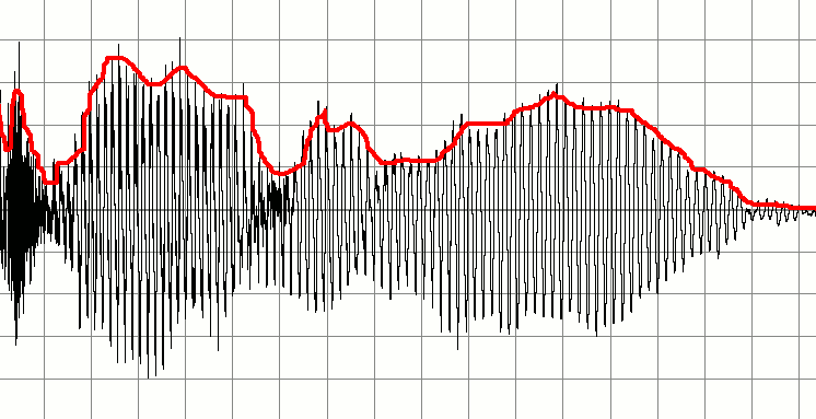
This is the simplest implementation, and probably the easiest to understand. A waveform is passed through a capacitor in a simple circuit, which charges whenever there is a high in the signal, and drains whenever there is a low. This allows it to create an almost sawtooth wave covering the envelope of a wave.

As seen above though, some issues arise in its implementation. The aggression of the fall in the created envelope depends on how fast the capacitor loses charge, so if it doesn’t lose charge fast enough, as seen above, there may be a large gap between the waveform dropping and the envelope following. This is still quite useful to consider, since it is easy to implement and reacts to rises immediately, so it may be usable given some modifications.

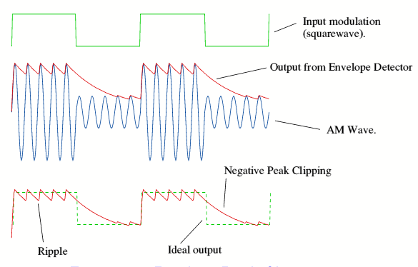
Rectifier and low-pass filter

This is where things get not-so-simple. Both this and the following method dive into some actual signal modulation to create an envelope from the original signal. I am also not the most knowledgable in this so please refer to this article’s header. From this point on, we get into signals. Most of the base information I got was from this MathWorks link. Beware.

This is the basic chain of this operation:

$$\text{Input} \rightarrow u^2 \rightarrow u*2 \rightarrow \text{Downsample} \rightarrow \text{LPF} \rightarrow \sqrt{u} \rightarrow \text{Output}$$

The input to this is the original sound waveform. This signal is rectified (or squared), to essentially make it its own carrier wave. Rectifying, for our understanding, mainly takes the loud sound wave and brings it back to a much smoother wave. From there, the signal is multiplied by 2 to help scale it up for processing, and downsampled. Downsampling removes some sampled data points, to simulate a lower sample rate and reduce the complexity of our resulting wave. Finally, a LPF, or Low Pass Filter is applied. A Low Pass Filter allows for low frequency waves, like our resulting wave, to pass through, and prevents high-frequency waves, like any small fast bumps in that wave, to be smoothed out. Finally, we take the square root of the resulting signal to scale it back down and match it to our original data.

This process definitely take some steps up in complexity, but it is really interesting on how it modulates the original waveform. Doing downsampling and (mainly) filtering in real time can sometimes be an issue in terms of delay, but this is something we can investigate. Essentially, this is a lot more accurate than our previous method, but a lot more expensive.

Hilbert Transform

I am going to save the deepdive on this. This is something you can check out on the original MathWorks link, but it is essentially a more grandiose version of our rectifier and LPF described above. This one is seriously impressive, but again, is more computationally expensive. The main problem is that a real time Hilbert Transform is a point of high-level research, and as well that its main focus is on waveforms without massive changes. This does not match our use case.

Really cool though.

What I would like to do

As mentioned above, each piece has their pros and cons. The main things I want to keep in mind though are the following:

• This is for a real-time sidechaining module, so delay would be easily noticeable, and the ideal case would be if we could even be early.
• This will be a VCV Rack module at the end of the day, so we will be sharing computer resources with a wide range of other modules. Something computationally expensive may be neat in its own physical module, but would be rude in this context.

With these in mind, I would mainly want to focus on an advanced version of the diode detector, maybe with some peak detection so we could be aware of jumps from high to low frequencies. The best way to discover what’s best would be through testing though, so that’s what’s next currently.

What I am doing

Note that this is a stream of consciousness as I’ve been updating the module over time.

Now, for setting up a testing environment on waveform manipulation, I highly recommend looking towards Python with Scipy and MatPlotLib, so you can easily adjust parameters and see how different functions work on different waveforms. I did not do this though because I like to dive directly into the use case and also I wanted to keep momentum on this project without getting slowed down from importing different .WAVs to test on.

So, alternatively, I have made a rough version of this future module to test directly in VCV Rack. I am also using VCV Rack’s Scope to view the waveform I am creating, as well as Audible Instrument’s Macro Oscillator 2 (or as many of us formally know it, Plaits).

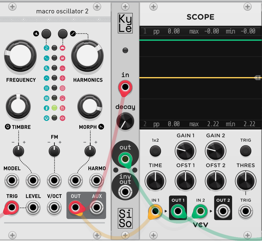
T1: Diode Detector with Rectifier

To start testing, the Kyle module was fitted with a diode detector implementation. This was obviously the easiest to implement, but it was also what I believed would be the closest to the final implementation of the model.

// Abs the current value, make all peaks positive
currVoltage = abs(inputs[SIGNAL_INPUT].getVoltage());
// Set the output
// If the signal is greater than the current output voltage
if (currVoltage > outVoltage)
{
    // Set the output to the signal voltage
    outVoltage = currVoltage;
}
// If the current output voltage is greater than the signal
else
{
    // Reduce the output by a given decay value
    outVoltage -= params[PDECAY_PARAM].getValue() / 1000;
}
// Set the output
outputs[ENV_OUTPUT].setVoltage(outVoltage);

I had set the module to take any signal as an input and rectify it so all peaks were positive. Then, as the signal is running, the module would either clone the signal if the voltage was higher than its current voltage, or decay at a constant amount, ranging from 0 to 1/1000 per sample, depending on the decay knob value.

The decay, as expected, was extremely rigid. Hugging a waveform without some sort of exponential decay would definitely be an issue down the line. We could introduce some complexity into how we handle change in the waveform such as…

• Exponential/logarithmic decay
• Decay based on current voltage (stronger at higher voltage, weaker at lower)
• Moving window decay (alternative of the above, looking at how radically the data changes over a certain historical period and adjusting the decay rate accordingly)

Furthermore, the rigid nature of the waveform seems to really come to a head at near-constant or low change areas of the signal waveform, namely at the low voltages of our test. This is somewhere that the current voltage decay basing and/or moving window could come in handy.

With all of this, the next implementation of the Kyle module would include some controls for toggling between exponential or linear decay, as well as altering decay based on current voltage. The moving window is something I find interesting, but will be looked at down the line if necessary.

T2: Diode Detector with Mass Adjustment Parameters

Next try, new controls! Things have gotten undeniably worse visually but that’s what prototyping is for! Added in now are controls to change the decay type between exponential, linear, and logarithmic, as well as a knob to control how much the current voltage affects how fast the decay takes place.

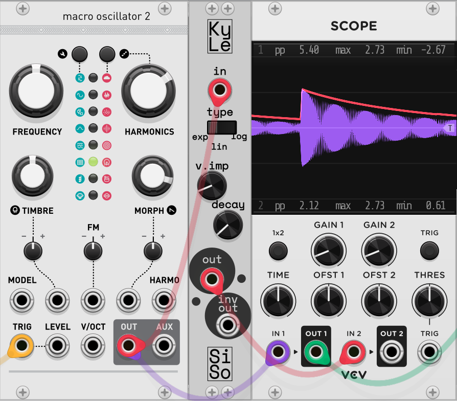
Some immediate roadblocks were shown, mainly in having a constant exponential or logarithmic decay. When tweaking the decay knob, you could get a good curve to hug any quickly dropping high peaks, but whenever the voltage reached much lower values than that peak, there would be a fuzz of the curve immediately dropping from the low voltage, to somewhere much lower than the original waveform, and then bouncing back up. This was the wake-up call that reminded me that I would need to make the exponential and logarithmic decays relative to the voltages of the original signal, rather than keep it as its own knob.

// Exponential, return function of time
float expDecay()
{
    // e^(t * decay) * currVoltage / 10
    return exp(t * (params[PDECAY_PARAM].getValue() * 10.f)) * (currVoltage / 7500.f);
}

// Linear, return constant decay
float linDecay()
{
    // linear, just decay
    return params[PDECAY_PARAM].getValue() / 1000.f;
}

// Logarithmic, return function of time
float logDecay()
{
    // log(t * decay) * currVoltage / 10
    return std::max(0.f, log(t * (params[PDECAY_PARAM].getValue() * 10.f)) * (currVoltage / 10.f));
}

I also realized that my terminology was off. The curves that I was looking to model in the decay were ones bowing inward and outwards, but the exp and log decay curves both curve outwards. To get the curves I wanted, I would be looking at an exp and inverse exp function. Because of this, and after some testing, I realized the UI could be better by having one knob control the acceleration of the curve while the other can scale the entire decay function:

$$\text{decay}*e^{\text{accel}}$$

The decay knob would stay as-is, and the selector would then be replaced by the acceleration knob, or what will likely just be labelled exp. The voltage impact knob as seen on this demo will be removed since it is unneeded.

Something else I was wondering about was if we used inverse exponential decay at high amplitudes and regular exponential decay at low amplitudes, but that may be more complicated than it’s worth and would need to introduce more controls. I’ll mainly be looking at how the above works in the next iteration.

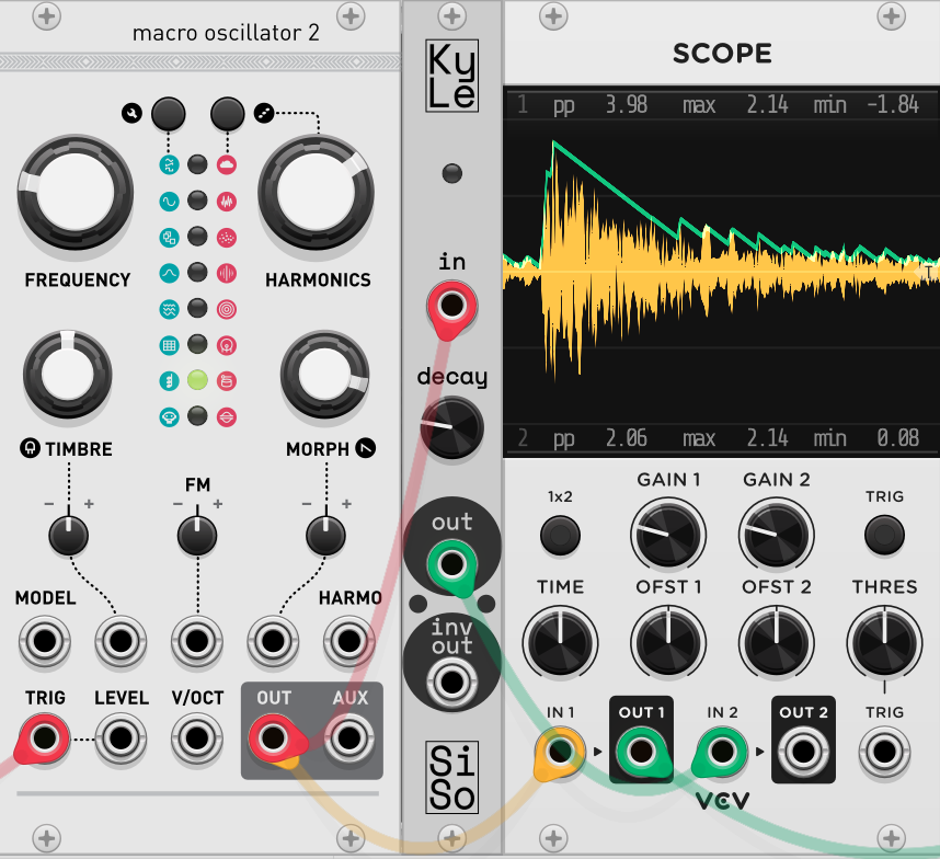
T3: Exponential Decay Diode Detector

IT MODERATELY WORKS! This is the first iteration that I am happy to use as a base to tweak for final release. Since the last try, I implemented the exp knob as described above. Negative values make it curve in while positive values make it curve out. I also added an amplification knob to multiply the output, allowing even small changes to be much more impactful for sidechain usage.

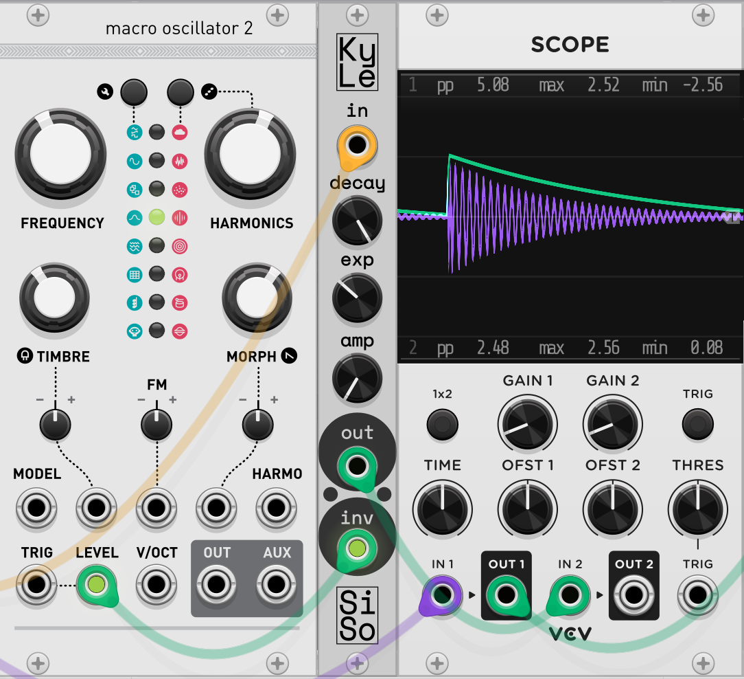
This time around, the code has gotten quite neat and compact, to the point I can put the whole process code here pretty comfortably. Some notable changes are now scaling the decay value in relation to the sample rate to keep things consistent at different values, as well as finally implementing the inverse envelope to allow for level/VCA modulation.

// Get input voltage (keep it positive)
currVoltage = abs(inputs[SIGNAL_INPUT].getVoltage());
// Add to the timer
t += args.sampleTime;

/*
    We decay the signal either exponentially if PEXP != 0,
    otherwise we decay linearly
    out - (decay * e^(exp))
*/
outVoltage = outVoltage - ((params[PDECAY_PARAM].getValue() / args.sampleRate) *
                            exp((params[PEXP_PARAM].getValue() * t)));

/*
    If the original signal is greater than our output voltage,
        currVoltage > outVoltage
    Set the output to the signal voltage. Otherwise, use the
    decayed output voltage
*/
if (currVoltage >= outVoltage)
{
    outVoltage = currVoltage;
    // Reset the time
    t = 0.f;
}
outVoltage = std::max(currVoltage, outVoltage);

// Amplify the output (maxing out at 10)
ampOut = std::min(10.f, abs(outVoltage * (1 + 9.f * params[PAMP_PARAM].getValue())));

// Set output voltages, accounting for amplification
outputs[ENV_OUTPUT].setVoltage(ampOut);
outputs[ENVINV_OUTPUT].setVoltage(10 - ampOut);

As usual, there is always more to fix and improve on.

Using a negative exponent is very cool for hugging a shrinking waveform without ever needing to hit that waveform until the next peak, but at high negative values and low decay values it does not converge to 0. This is also seen with a constant decay and decay set to 0. This could likely be fixed by checking if the input has been at or around 0 for a number of samples, and/or if anything is plugged into the unit. If this is the case, we can slowly decay the value to 0 or just jump it.

As mentioned in the last iteration, there could be a use for using both positive and negative exponential decay values depending on the current voltage of the signal, but I will likely leave that for a revamp of the module in the future (which I can then change $20 more for).

I was also thinking of the possibility of adding a max and min value, scaling all voltages from the original signal above max to an output of 10V, all voltages below min to an output of 0V, and appropriately matching the central values. I’m gonna run this all by some people to see how useful it could be and if it’s worthwhile to implement.

The final thing to touch upon would probably be some iconography to help visually explain what different exponent values and even amplification values mean, there’s enough room for it too so why not.

Where from here

I think Kyle has reached a stable enough point for a base release, with a lot to think on for a future refactor. Once this module releases, the Kyle, Sesame, and Lola modules will all be reviewed to add in any extra features as well as resource test to confirm they’ll work well in VCV Rack. Finally, assuming all this goes well, they’ll be submitted to the VCV Library. Until then, I write.